VCE General Maths Data Analysis 2020 Mini Test 2
VCAA General Maths Exam 2
This is the full VCE General Maths Exam with worked solutions. You can also try Mini-Tests, which are official VCAA exams split into short tests you can do anytime.
Number of marks: 12
Reading time: 2 minutes
Writing time: 18 minutes
Instructions
• Answer all questions in the spaces provided.
• Write your responses in English.
• In all questions where a numerical answer is required, you should only round your answer when instructed to do so.
• Unless otherwise indicated, the diagrams in this book are not drawn to scale.
Data analysis - 2020 - Exam 2 (Part 2)
The scatterplot below shows body density, in kilograms per litre, plotted against waist measurement, in centimetres, for 250 men.
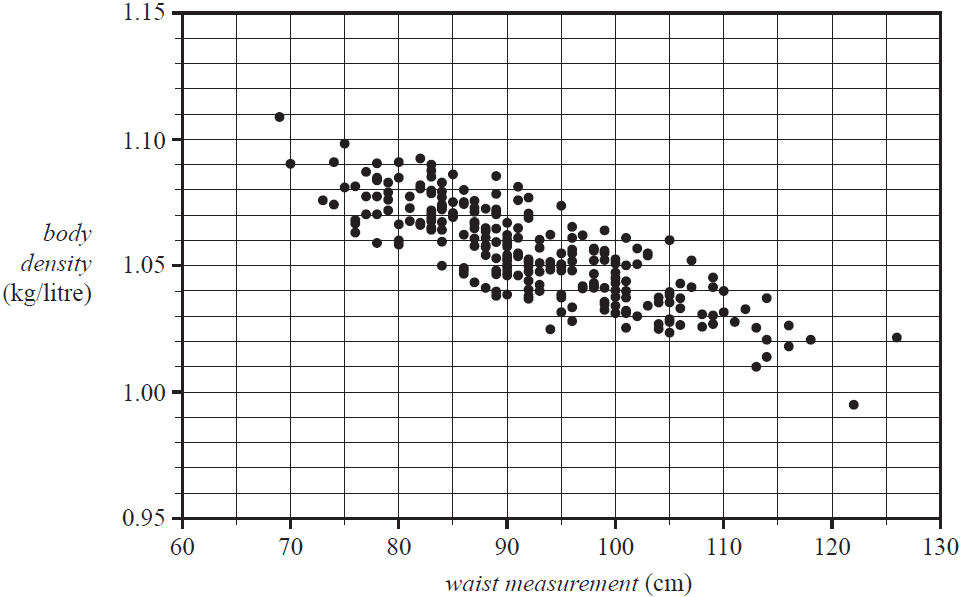
When a least squares line is fitted to the scatterplot, the equation of this line is
\( \textit{body density} = 1.195 - 0.001512 \times \textit{waist measurement} \)
a. Draw the graph of this least squares line on the scatterplot above. 1 mark
b. Use the equation of this least squares line to predict the body density of a man whose waist measurement is 65 cm.
Round your answer to two decimal places. 1 mark
c. When using the equation of this least squares line to make the prediction in part b., are you extrapolating or interpolating? 1 mark
d. Interpret the slope of this least squares line in terms of a man’s body density and waist measurement. 1 mark
e. In this study, the body density of the man with a waist measurement of 122 cm was 0.995 kg/litre.
Show that, when this least squares line is fitted to the scatterplot, the residual, rounded to two decimal places, is –0.02. 1 mark
f. The coefficient of determination for this data is 0.6783.
Write down the value of the correlation coefficient \(r\).
Round your answer to three decimal places. 1 mark
g. The residual plot associated with fitting a least squares line to this data is shown below.
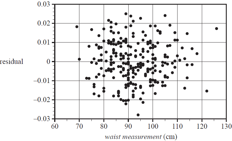
Does this residual plot support the assumption of linearity that was made when fitting this line to this data? Briefly explain your answer. 1 mark
The age, in years, body density, in kilograms per litre, and weight, in kilograms, of a sample of 12 men aged 23 to 25 years are shown in the table below.
| Age (years) |
Body density (kg/litre) |
Weight (kg) |
|---|---|---|
| 23 | 1.07 | 70.1 |
| 23 | 1.07 | 90.4 |
| 23 | 1.08 | 73.2 |
| 23 | 1.08 | 85.0 |
| 24 | 1.03 | 84.3 |
| 24 | 1.05 | 95.6 |
| 24 | 1.07 | 71.7 |
| 24 | 1.06 | 95.0 |
| 25 | 1.07 | 80.2 |
| 25 | 1.09 | 87.4 |
| 25 | 1.02 | 94.9 |
| 25 | 1.09 | 65.3 |
a. For these 12 men, determine
i. their median age, in years 1 mark
ii. the mean of their body density, in kilograms per litre. 1 mark
b. A least squares line is to be fitted to the data with the aim of predicting body density from weight.
i. Name the explanatory variable for this least squares line. 1 mark
ii. Determine the slope of this least squares line.
Round your answer to three significant figures. 1 mark
c. What percentage of the variation in body density can be explained by the variation in weight? Round your answer to the nearest percentage. 1 mark
End of Multiple-Choice Question Book
VCE is a registered trademark of the VCAA. The VCAA does not endorse or make any warranties regarding this study resource. Past VCE exams and related content can be accessed directly at www.vcaa.vic.edu.au