2018 VCE Further Maths Exam 2
This is the full VCE Further Maths Exam with worked solutions. You can also try Mini-Tests, which are official VCAA exams split into short tests you can do anytime.
Number of marks: 60
Reading time: 15 minutes
Writing time: 1.5 hours
Instructions
• Answer all questions in pencil on your Multiple-Choice Answer Sheet.
• Choose the response that is correct for the question.
• A correct answer scores 1; an incorrect answer scores 0.
• Marks will not be deducted for incorrect answers.
• No marks will be given if more than one answer is completed for any question.
• Unless otherwise indicated, the diagrams in this book are not drawn to scale.
SECTION A – Core
Data analysis
Question 1 (8 marks)Table 1
| City | Congestion level |
Size | Increase in travel time (minutes per day) |
|---|---|---|---|
| Belfast | high | small | 52 |
| Edinburgh | high | small | 43 |
| London | high | large | 40 |
| Manchester | high | large | 44 |
| Brighton and Hove | high | small | 35 |
| Bournemouth | high | small | 36 |
| Sheffield | medium | small | 36 |
| Hull | medium | small | 40 |
| Bristol | medium | small | 39 |
| Newcastle-Sunderland | medium | large | 34 |
| Leicester | medium | small | 36 |
| Liverpool | medium | large | 29 |
| Swansea | low | small | 30 |
| Glasgow | low | large | 34 |
| Cardiff | low | small | 31 |
| Nottingham | low | small | 31 |
| Birmingham-Wolverhampton | low | large | 29 |
| Leeds-Bradford | low | large | 31 |
| Portsmouth | low | small | 27 |
| Southampton | low | small | 30 |
| Reading | low | small | 31 |
| Coventry | low | small | 30 |
| Stoke-on-Trent | low | small | 29 |
The data in Table 1 on page 2 relates to the impact of traffic congestion in 2016 on travel times in 23 cities in the United Kingdom (UK).
The four variables in this data set are:
- city – name of city
- congestion level – traffic congestion level (high, medium, low)
- size – size of city (large, small)
- increase in travel time – increase in travel time due to traffic congestion (minutes per day).
a. How many variables in this data set are categorical variables? 1 mark
b. How many variables in this data set are ordinal variables? 1 mark
c. Name the large UK cities with a medium level of traffic congestion. 1 mark
d. Use the data in Table 1 to complete the following two-way frequency table, Table 2. 2 marks
Table 2
| Congestion level | City size | |
|---|---|---|
| Small | Large | |
| high | 4 | |
| medium | ||
| low | ||
| Total | 16 | |
e. What percentage of the small cities have a high level of traffic congestion? 1 mark
Traffic congestion can lead to an increase in travel times in cities. The dot plot and boxplot below both show the increase in travel time due to traffic congestion, in minutes per day, for the 23 UK cities.
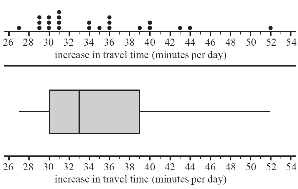
f. Describe the shape of the distribution of the increase in travel time for the 23 cities. 1 mark
g. The data value 52 is below the upper fence and is not an outlier.
Determine the value of the upper fence. 1 mark
The congestion level in a city can also be recorded as the percentage increase in travel time due to traffic congestion in peak periods (compared to non-peak periods).
This is called the percentage congestion level.
The percentage congestion levels for the morning and evening peak periods for 19 large cities are plotted on the scatterplot below.
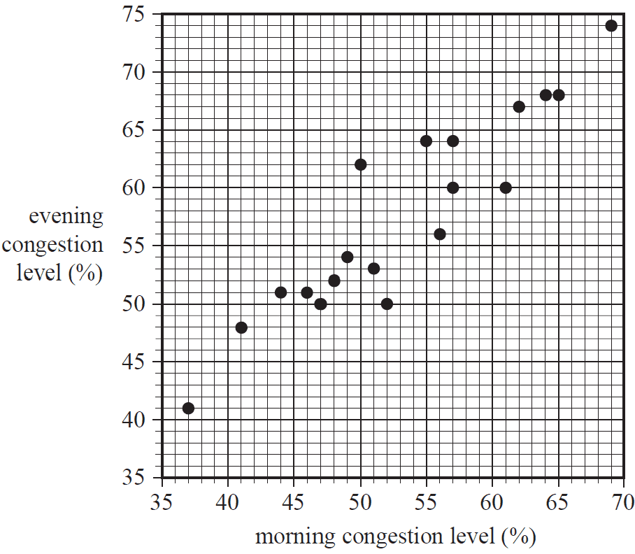
a. Determine the median percentage congestion level for the morning peak period and the evening peak period.
Write your answers in the appropriate boxes provided below. 2 marks
Median percentage congestion level for morning peak period %
Median percentage congestion level for evening peak period %
A least squares line is to be fitted to the data with the aim of predicting evening congestion level from morning congestion level.
The equation of this line is
evening congestion level = \(8.48 + 0.922 \times\) morning congestion level
b. Name the response variable in this equation. 1 mark
c. Use the equation of the least squares line to predict the evening congestion level when the morning congestion level is 60%. 1 mark
d. Determine the residual value when the equation of the least squares line is used to predict the evening congestion level when the morning congestion level is 47%.
Round your answer to one decimal place. 2 marks
e. The value of the correlation coefficient \(r\) is 0.92.
What percentage of the variation in the evening congestion level can be explained by the variation in the morning congestion level?
Round your answer to the nearest whole number. 1 mark
Table 3 shows the yearly average traffic congestion levels in two cities, Melbourne and Sydney, during the period 2008 to 2016. Also shown is a time series plot of the same data.
The time series plot for Melbourne is incomplete.
Table 3
| Year | Congestion level (%) | ||||||||
|---|---|---|---|---|---|---|---|---|---|
| 2008 | 2009 | 2010 | 2011 | 2012 | 2013 | 2014 | 2015 | 2016 | |
| Melbourne | 25 | 26 | 26 | 27 | 28 | 28 | 28 | 29 | 33 |
| Sydney | 28 | 30 | 32 | 33 | 34 | 34 | 35 | 36 | 39 |
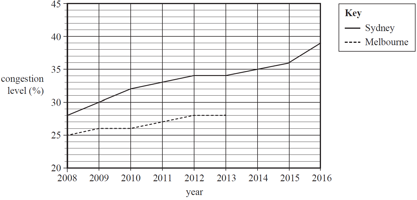
a. Use the data in Table 3 to complete the time series plot above for Melbourne. 1 mark
(Answer on the time series plot above.)
b. A least squares line is used to model the trend in the time series plot for Sydney. The equation is
congestion level = \(-2280 + 1.15 \times\) year
i. Draw this least squares line on the time series plot on page 8. 1 mark
(Answer on the time series plot on page 8.)
ii. Use the equation of the least squares line to determine the average rate of increase in percentage congestion level for the period 2008 to 2016 in Sydney.
Write your answer in the box provided below. 1 mark
% per year
iii. Use the least squares line to predict when the percentage congestion level in Sydney will be 43%. 1 mark
The yearly average traffic congestion level data for Melbourne is repeated in Table 4 below.
Table 4
| Year | Congestion level (%) | ||||||||
|---|---|---|---|---|---|---|---|---|---|
| 2008 | 2009 | 2010 | 2011 | 2012 | 2013 | 2014 | 2015 | 2016 | |
| Melbourne | 25 | 26 | 26 | 27 | 28 | 28 | 28 | 29 | 33 |
c. When a least squares line is used to model the trend in the data for Melbourne, the intercept of this line is approximately \(-1514.75556\).
Round this value to four significant figures. 1 mark
d. Use the data in Table 4 to determine the equation of the least squares line that can be used to model the trend in the data for Melbourne. The variable year is the explanatory variable.
Write the values of the intercept and the slope of this least squares line in the appropriate boxes provided below.
Round both values to four significant figures. 2 marks
congestion level = + \(\times\) year
e. Since 2008, the equations of the least squares lines for Sydney and Melbourne have predicted that future traffic congestion levels in Sydney will always exceed future traffic congestion levels in Melbourne.
Explain why, quoting the values of appropriate statistics. 2 marks
Recursion and financial modelling
Question 4 (5 marks)Julie deposits some money into a savings account that will pay compound interest every month.
The balance of Julie's account, in dollars, after \(n\) months, \(V_n\), can be modelled by the recurrence relation shown below.
\(V_0 = 12000, \quad V_{n+1} = 1.0062 V_n\)
a. How many dollars does Julie initially invest? 1 mark
b. Recursion can be used to calculate the balance of the account after one month.
i. Write down a calculation to show that the balance in the account after one month, \(V_1\), is $12074.40. 1 mark
ii. After how many months will the balance of Julie's account first exceed $12300? 1 mark
c. A rule of the form \(V_n = a \times b^n\) can be used to determine the balance of Julie's account after \(n\) months.
i. Complete this rule for Julie's investment after \(n\) months by writing the appropriate numbers in the boxes provided below. 1 mark
balance = \(\times\) \(^n\)
ii. What would be the value of \(n\) if Julie wanted to determine the value of her investment after three years? 1 mark
After three years, Julie withdraws $14000 from her account to purchase a car for her business.
For tax purposes, she plans to depreciate the value of her car using the reducing balance method.
The value of Julie's car, in dollars, after \(n\) years, \(C_n\), can be modelled by the recurrence relation shown below.
\(C_0 = 14000, \quad C_{n+1} = R \times C_n\)
a. For each of the first three years of reducing balance depreciation, the value of \(R\) is 0.85.
What is the annual rate of depreciation in the value of the car during these three years? 1 mark
b. For the next five years of reducing balance depreciation, the annual rate of depreciation in the value of the car is changed to 8.6%.
What is the value of the car eight years after it was purchased?
Round your answer to the nearest cent. 2 marks
Julie has retired from work and has received a superannuation payment of $492 800.
She has two options for investing her money.
Option 1
Julie could invest the $492 800 in a perpetuity. She would then receive $887.04 each fortnight for the rest of her life.
a. At what annual percentage rate is interest earned by this perpetuity? 1 mark
Option 2
Julie could invest the $492 800 in an annuity, instead of a perpetuity.
The annuity earns interest at the rate of 4.32% per annum, compounding monthly.
The balance of Julie's annuity at the end of the first year of investment would be $480 242.25
b.
i. What monthly payment, in dollars, would Julie receive? 1 mark
ii. How much interest would Julie's annuity earn in the second year of investment?
Round your answer to the nearest cent. 2 marks
SECTION B – Modules
Module 1 – Matrices
Question 1 (3 marks)A toll road is divided into three sections, \(E\), \(F\) and \(G\).
The cost, in dollars, to drive one journey on each section is shown in matrix \(C\) below.
\[ C = \begin{bmatrix} 3.58 \\ 2.22 \\ 2.87 \end{bmatrix} \begin{matrix} E \\ F \\ G \end{matrix} \]
a. What is the cost of one journey on section \(G\)? 1 mark
b. Write down the order of matrix \(C\). 1 mark
c. One day Kim travels once on section \(E\) and twice on section \(G\).
His total toll cost for this day can be found by the matrix product \(M \times C\).
Write down the matrix \(M\). 1 mark
\(M\) =
The Westhorn Council must prepare roads for expected population changes in each of three locations: main town (\(M\)), villages (\(V\)) and rural areas (\(R\)).
The population of each of these locations in 2018 is shown in matrix \(P_{2018}\) below.
\[ P_{2018} = \begin{bmatrix} 2100 \\ 1800 \\ 1700 \end{bmatrix} \begin{matrix} M \\ V \\ R \end{matrix} \]
The expected annual change in population in each location is shown in the table below.
| Location | main town | villages | rural areas |
| Annual change | increase by 4% | decrease by 1% | decrease by 2% |
a. Write down matrix \(P_{2019}\), which shows the expected population in each location in 2019. 1 mark
\(P_{2019}\) =
b. The expected population in each of the three locations in 2019 can be determined from the matrix product
\(P_{2019} = F \times P_{2018}\)
where \(F\) is a diagonal matrix.
Write down matrix \(F\). 1 mark
\(F\) =
The Hiroads company has a contract to maintain and improve 2700 km of highway.
Each year sections of highway must be graded (\(G\)), resurfaced (\(R\)) or sealed (\(S\)).
The remaining highway will need no maintenance (\(N\)) that year.
Let \(S_n\) be the state matrix that shows the highway maintenance schedule for the \(n\)th year after 2018.
The maintenance schedule for 2018 is shown in matrix \(S_0\) below.
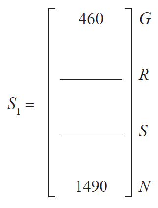
\[ S_0 = \begin{bmatrix} 700 \\ 400 \\ 200 \\ 1400 \end{bmatrix} \begin{matrix} G \\ R \\ S \\ N \end{matrix} \]
The type of maintenance in sections of highway varies from year to year, as shown in the transition matrix, \(T\), below.
\[ T = \begin{array}{cc} & \begin{array}{cccc} \textit{this year} \end{array} \\ & \begin{array}{cccc} G & R & S & N \end{array} \\ \begin{matrix} G \\ R \\ S \\ N \end{matrix} & \left[ \begin{array}{cccc} 0.2 & 0.1 & 0.0 & 0.2 \\ 0.1 & 0.1 & 0.0 & 0.2 \\ 0.2 & 0.1 & 0.2 & 0.1 \\ 0.5 & 0.7 & 0.8 & 0.5 \end{array} \right] \end{array} \begin{array}{c} \textit{next year} \end{array} \]
a. Of the length of highway that was graded (\(G\)) in 2018, how many kilometres are expected to be resurfaced (\(R\)) the following year? 1 mark
b. Show that the length of highway that is to be graded (\(G\)) in 2019 is 460 km by writing the appropriate numbers in the boxes below. 1 mark
\(\times\) 700 + \(\times\) 400 + \(\times\) 200 + \(\times\) 1400 = 460
The state matrix describing the highway maintenance schedule for the \(n\)th year after 2018 is given by
\(S_{n+1} = T S_n\)
c. Complete the state matrix, \(S_1\), below for the highway maintenance schedule for 2019 (one year after 2018). 1 mark
d. In 2020, 1536 km of highway is expected to require no maintenance (\(N\)).
Of these kilometres, what percentage is expected to have had no maintenance (\(N\)) in 2019?
Round your answer to one decimal place. 1 mark
e. In the long term, what percentage of highway each year is expected to have no maintenance (\(N\))?
Round your answer to one decimal place. 1 mark
Beginning in the year 2021, a new company will take over maintenance of the same 2700 km highway with a new contract.
Let \(M_n\) be the state matrix that shows the highway maintenance schedule of this company for the \(n\)th year after 2020.
The maintenance schedule for 2020 is shown in matrix \(M_0\) below.
For these 2700 km of highway, the matrix recurrence relation shown below can be used to determine the number of kilometres of this highway that will require each type of maintenance from year to year.
\(M_{n+1} = T M_n + B\)
where
\[ M_0 = \begin{bmatrix} 500 \\ 400 \\ 300 \\ 1500 \end{bmatrix} \begin{matrix} G \\ R \\ S \\ N \end{matrix}, \quad T = \begin{array}{cc} & \begin{array}{cccc} \textit{this year} \end{array} \\ & \begin{array}{cccc} G & R & S & N \end{array} \\ \begin{matrix} G \\ R \\ S \\ N \end{matrix} & \left[ \begin{array}{cccc} 0.2 & 0.1 & 0.0 & 0.2 \\ 0.1 & 0.1 & 0.0 & 0.2 \\ 0.2 & 0.1 & 0.2 & 0.1 \\ 0.5 & 0.7 & 0.8 & 0.5 \end{array} \right] \end{array} \begin{array}{c} \textit{next year} \end{array}, \quad B = \begin{bmatrix} k \\ 20 \\ 10 \\ -60 \end{bmatrix} \]
a. Write down the value of \(k\) in matrix \(B\). 1 mark
b. How many kilometres of highway are expected to be graded (\(G\)) in the year 2022? 1 mark
Module 2 – Networks and decision mathematics
Question 1 (3 marks)The graph below shows the possible number of postal deliveries each day between the Central Mail Depot and the Zenith Post Office.
The unmarked vertices represent other depots in the region.
The weighting of each edge represents the maximum number of deliveries that can be made each day.
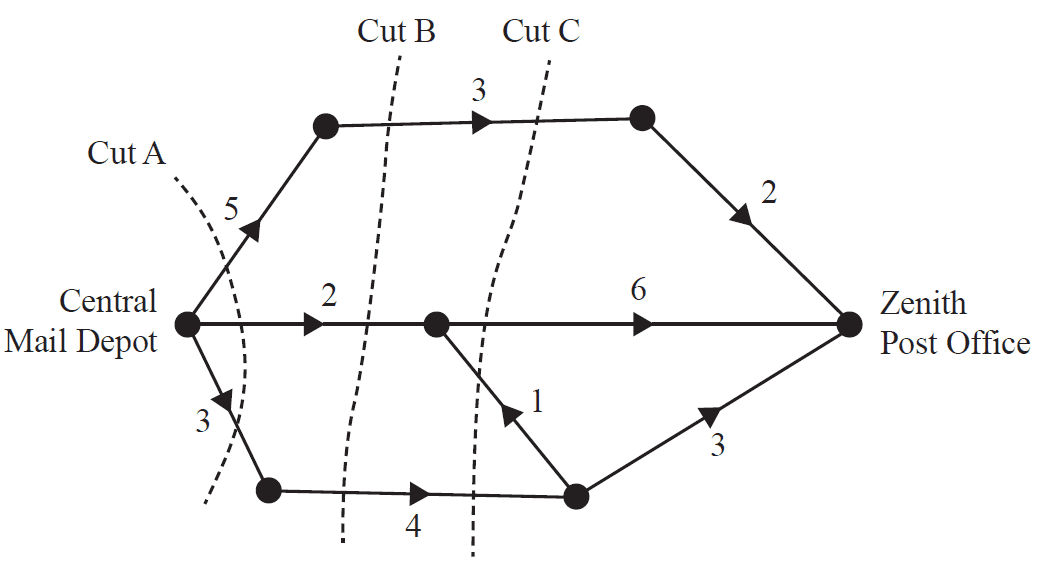
a. Cut A, shown on the graph, has a capacity of 10.
Two other cuts are labelled as Cut B and Cut C.
i. Write down the capacity of Cut B. 1 mark
ii. Write down the capacity of Cut C. 1 mark
b. Determine the maximum number of deliveries that can be made each day from the Central Mail Depot to the Zenith Post Office. 1 mark
In one area of the town of Zenith, a postal worker delivers mail to 10 houses labelled as vertices \(A\) to \(J\) on the graph below.
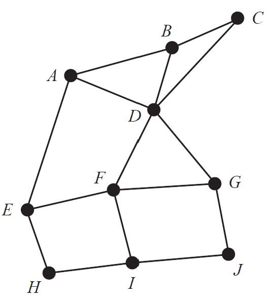
a. Which one of the vertices on the graph has degree 4? 1 mark
For this graph, an Eulerian trail does not currently exist.
b. For an Eulerian trail to exist, what is the minimum number of extra edges that the graph would require? 1 mark
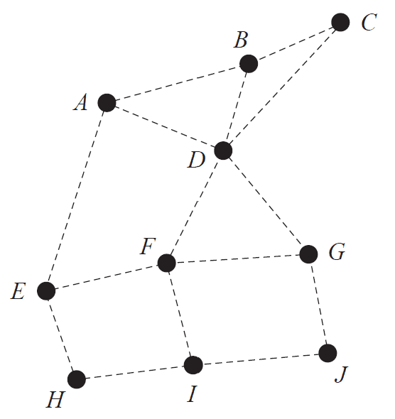
c. The postal worker has delivered the mail at \(F\) and will continue her deliveries by following a Hamiltonian path from \(F\).
Draw in a possible Hamiltonian path for the postal worker on the diagram below. 1 mark
At the Zenith Post Office all computer systems are to be upgraded.
This project involves 10 activities, \(A\) to \(J\).
The directed network below shows these activities and their completion times, in hours.
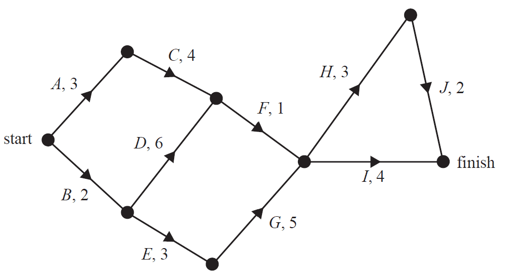
a. Determine the earliest starting time, in hours, for activity \(I\). 1 mark
b. The minimum completion time for the project is 15 hours.
Write down the critical path. 1 mark
c. Two of the activities have a float time of two hours.
Write down these two activities. 1 mark
d. For the next upgrade, the same project will be repeated but one extra activity will be added.
This activity has a duration of one hour, an earliest starting time of five hours and a latest starting time of 12 hours.
Complete the following sentence by filling in the boxes provided. 1 mark
The extra activity could be represented on the network above by a directed edge from the
end of activity to the start of activity .
Parcel deliveries are made between five nearby towns, \(P\) to \(T\).
The roads connecting these five towns are shown on the graph below. The distances, in kilometres, are also shown.
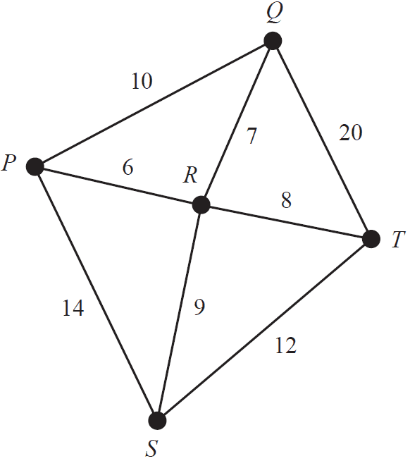
A road inspector will leave from town \(P\) to check all the roads and return to town \(P\) when the inspection is complete. He will travel the minimum distance possible.
a. How many roads will the inspector have to travel on more than once? 1 mark
b. Determine the minimum distance, in kilometres, that the inspector will travel. 1 mark
Module 3 – Geometry and measurement
Question 1 (5 marks)Tennis balls are packaged in cylindrical containers.
Frank purchases a container of tennis balls that holds three standard tennis balls, stacked one on top of the other.
This container has a radius of 3.4 cm and a height of 20.4 cm, as shown in the diagram below.
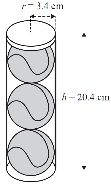
a. What is the diameter, in centimetres, of this container? 1 mark
b. What is the total outside surface area of this container, including both ends?
Write your answer in square centimetres, rounded to one decimal place. 1 mark
A standard tennis ball is spherical in shape with a radius of 3.4 cm.
c.
i. Write a calculation that shows that the volume, rounded to one decimal place, of one standard tennis ball is 164.6 cm³. 1 mark
ii. Write a calculation that shows that the volume, rounded to one decimal place, of the cylindrical container that can hold three standard tennis balls is 740.9 cm³. 1 mark
iii. How much unused volume, in cubic centimetres, surrounds the tennis balls in this container?
Round your answer to the nearest whole number. 1 mark
Frank travelled from Melbourne (38° S, 145° E) to a tennis tournament in Ho Chi Minh City, Vietnam, (11° N, 107° E).
Frank departed Melbourne at 10.30 pm on Monday, 5 February 2018.
Frank arrived in Ho Chi Minh City at 8.00 am on Tuesday, 6 February 2018.
The time difference between Melbourne and Ho Chi Minh City is four hours.
a. How long did it take Frank to travel from Melbourne to Ho Chi Minh City?
Give your answer in hours and minutes. 1 mark
Ho Chi Minh City is located at latitude 11° N and longitude 107° E.
Assume that the radius of Earth is 6400 km.
b.
i. Write a calculation that shows that the radius of the small circle of Earth at latitude 11° N is 6282 km, rounded to the nearest kilometre. 1 mark
ii. Iloilo City, in the Philippines, is located at latitude 11° N and longitude 123° E.
Find the shortest small circle distance between Ho Chi Minh City and Iloilo City.
Round your answer to the nearest kilometre. 1 mark
Frank owns a tennis court.
A diagram of his tennis court is shown below.
Assume that all intersecting lines meet at right angles.
Frank stands at point A. Another point on the court is labelled point B.
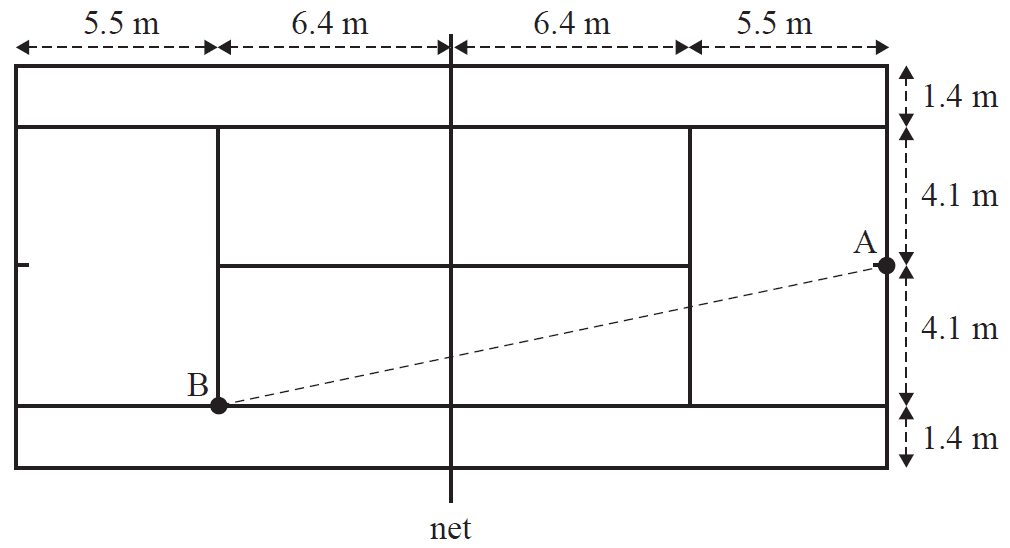
a. What is the straight-line distance, in metres, between point A and point B?
Round your answer to one decimal place. 1 mark
b. Frank hits a ball when it is at a height of 2.5 m directly above point A.
Assume that the ball travels in a straight line to the ground at point B.
What is the straight-line distance, in metres, that the ball travels?
Round your answer to the nearest whole number. 1 mark
c. Frank hits two balls from point A.
For Frank's first hit, the ball strikes the ground at point P, 20.7 m from point A.
For Frank's second hit, the ball strikes the ground at point Q.
Point Q is \(x\) metres from point A.
Point Q is 10.4 m from point P.
The angle, PAQ, formed is 23.5°.
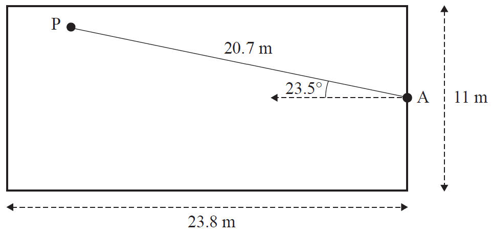
i. Determine two possible values for angle AQP.
Round your answers to one decimal place. 1 mark
ii. If point Q is within the boundary of the court, what is the value of \(x\)?
Round your answer to the nearest metre. 1 mark
Module 4 – Graphs and relations
Question 1 (2 marks)The following chart displays the daily gold prices (dollars per gram) for the month of November 2017.
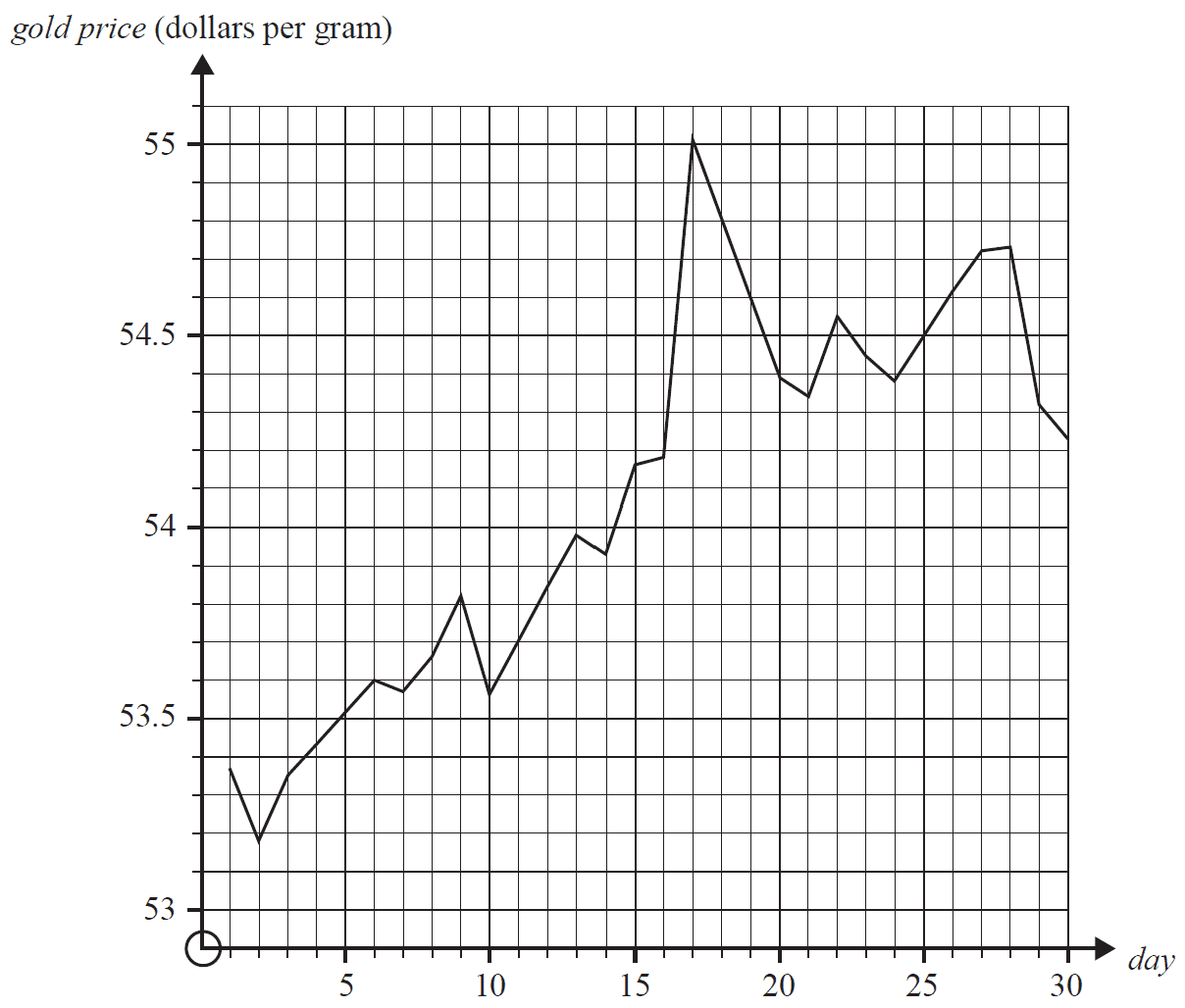
a. Which day in November had the lowest gold price? 1 mark
b. Between which two consecutive days did the greatest increase in gold price occur? 1 mark
The weight of gold can be recorded in either grams or ounces.
The following graph shows the relationship between weight in grams and weight in ounces.
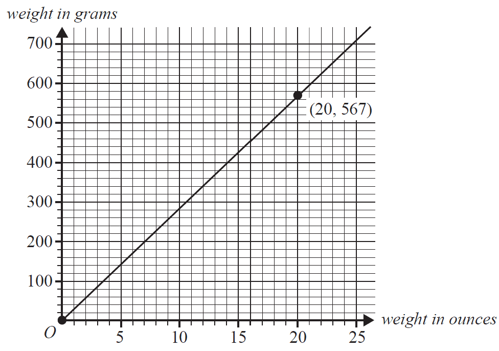
The relationship between weight measured in grams and weight measured in ounces is shown in the equation
weight in grams = \(M \times\) weight in ounces
a. Show that \(M = 28.35\). 1 mark
b. Robert found a gold nugget weighing 0.2 ounces.
Using the equation above, calculate the weight, in grams, of this gold nugget. 1 mark
c. Last year Robert sold gold to a buyer at $55 per gram.
The buyer paid Robert a total of $12 474.
Using the equation above, calculate the weight, in ounces, of this gold. 1 mark
Robert wants to hire a geologist to help him find potential gold locations.
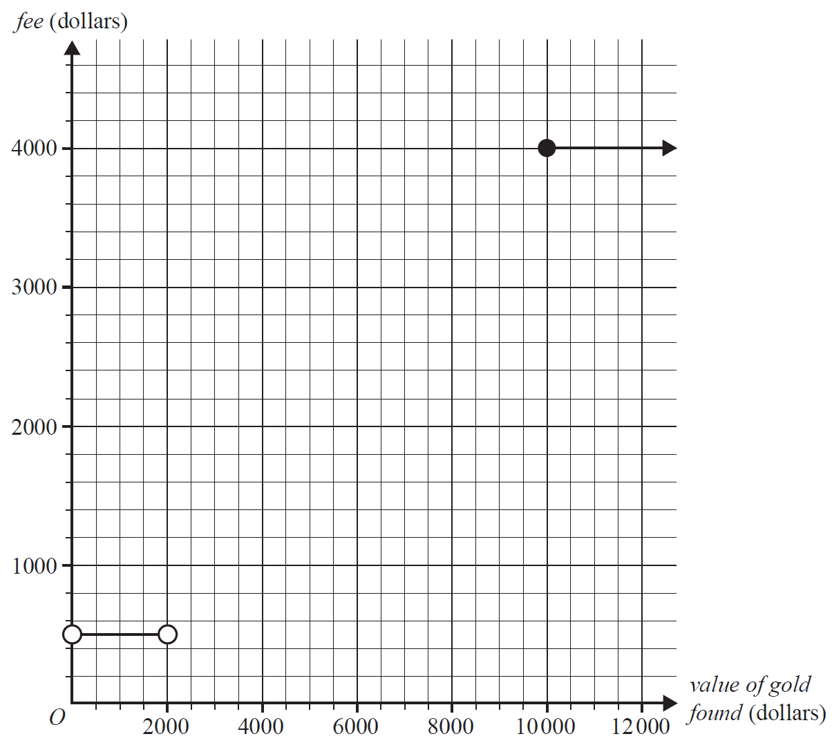
One geologist, Jennifer, charges a flat fee of $600 plus 25% commission on the value of gold found.
The following graph displays Jennifer's total fee in dollars.
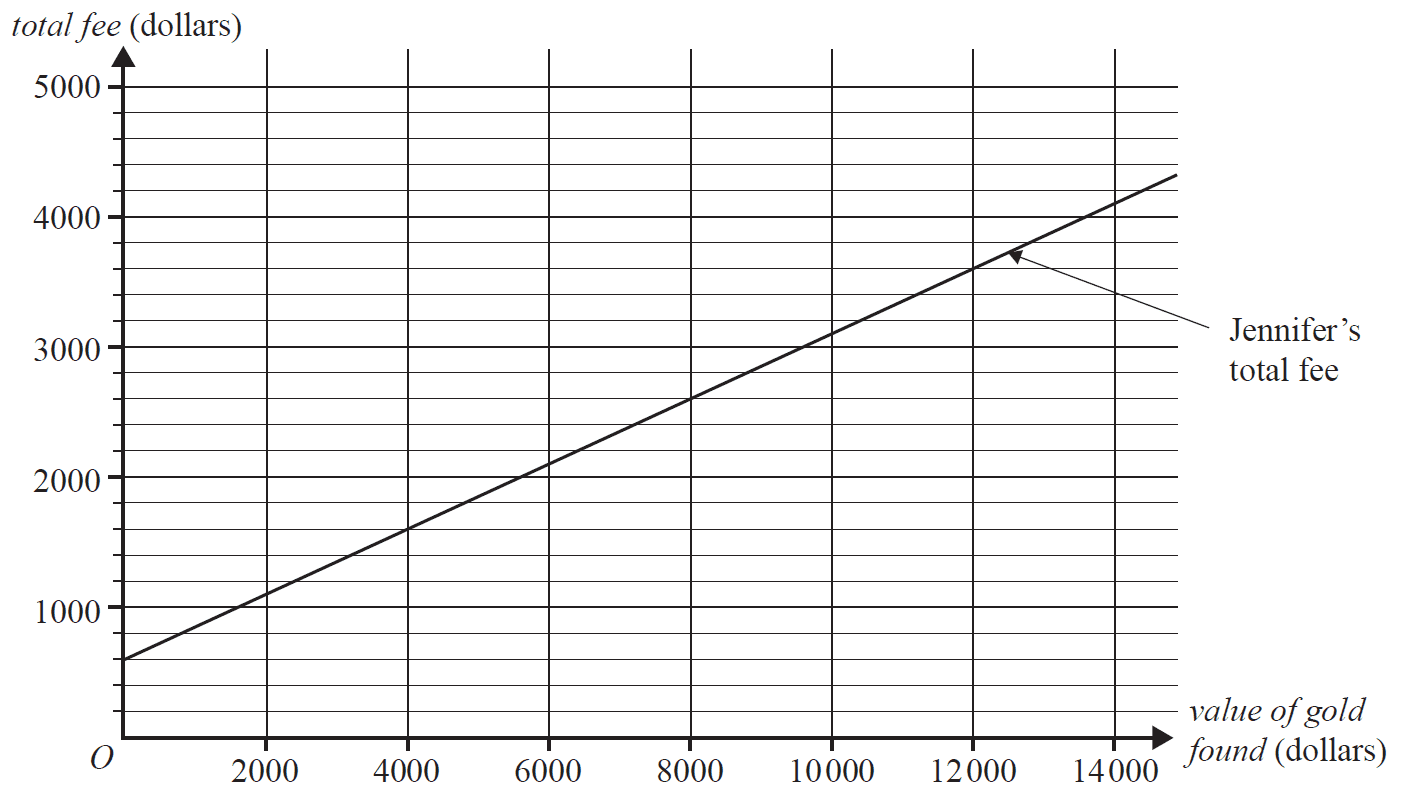
Another geologist, Kevin, charges a total fee of $3400 for the same task.
a. Draw a graph of the line representing Kevin's fee on the axes above. 1 mark
(Answer on the axes above.)
b. For what value of gold found will Kevin and Jennifer charge the same amount for their work? 1 mark
c. A third geologist, Bella, has offered to assist Robert.
Below is the relation that describes Bella's fee, in dollars, for the value of gold found.
\[ \text{fee (dollars)} = \begin{cases} 500 & 0 < \text{value of gold found} < 2000 \\ 1000 & 2000 \le \text{value of gold found} < 6000 \\ 2600 & 6000 \le \text{value of gold found} < 10000 \\ 4000 & \text{value of gold found} \ge 10000 \end{cases} \]
The step graph below representing this relation is incomplete.
Complete the step graph by sketching the missing information. 2 marks
This year Robert is planning a camping trip for the members of his gold prospecting club.
The club has chosen two camp sites, Bushman's Track and Lower Creek.
- Let \(x\) be the number of members staying at Bushman's Track.
- Let \(y\) be the number of members staying at Lower Creek.
- A maximum of 10 members can stay at Bushman's Track.
- A maximum of 15 members can stay at Lower Creek.
- At least 20 members in total are attending the camping trip.
The club has decided that at least twice as many members must stay at Lower Creek than at Bushman's Track.
These constraints can be represented by the following four inequalities.
Inequality 1 \(x \le 10\)
Inequality 2 \(y \le 15\)
Inequality 3 \(x + y \ge 20\)
Inequality 4 \(y \ge 2x\)
The graph below shows the four lines representing Inequalities 1 to 4.
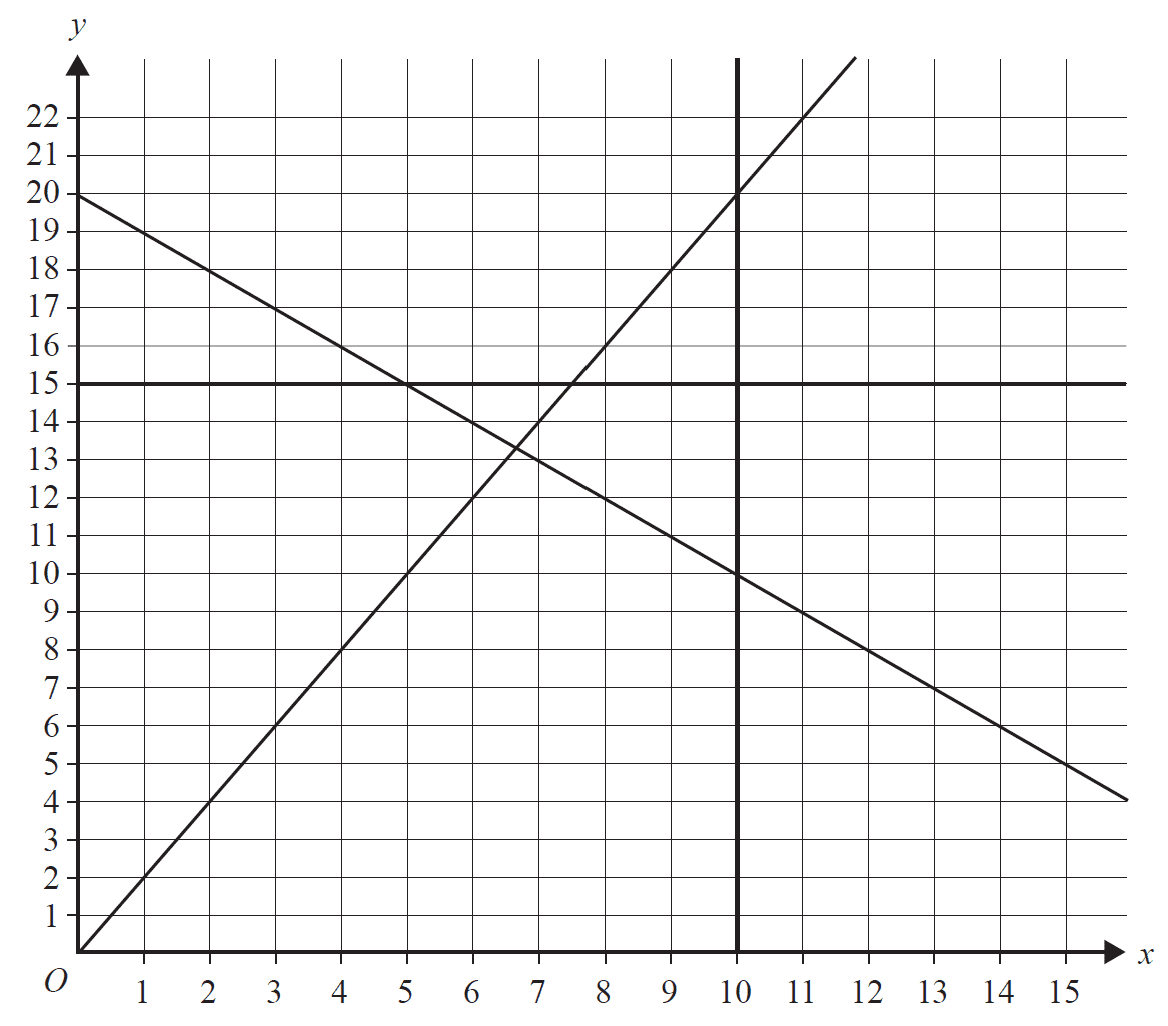
a. On the graph above, mark with a cross (×) the five integer points that satisfy Inequalities 1 to 4. 1 mark
(Answer on the graph above.)
The cost for one member to stay at Bushman's Track is $130. The cost for one member to stay at Lower Creek is $110.
For budgeting purposes, Robert needs to know the maximum cost of accommodation for both camp sites given Inequalities 1 to 4.
b. Find the total maximum cost of accommodation. 1 mark
c. When Robert finally made the booking, he was informed that, due to recent renovations, there were two changes to the accommodation at Lower Creek:
- A maximum of 22 members can now stay at Lower Creek.
- The cost for one member to stay at Lower Creek is now $140.
Twenty members will be attending the camping trip.
Find the total minimum cost of accommodation for these 20 members. 1 mark
End of Multiple-Choice Question Book
VCE is a registered trademark of the VCAA. The VCAA does not endorse or make any warranties regarding this study resource. Past VCE exams and related content can be accessed directly at www.vcaa.vic.edu.au