2023 SACE Stage 2 Maths Methods Exam Paper
Question Book 1 & Question Book 2
This is a full SACE Stage 2 Maths Methods Exam with worked solutions. You can also try Mini-Tests, which are official SACE exams split into short tests you can do anytime.
Number of marks: 100
Writing time: 130 minutes
Instructions
• Show appropriate working and steps of logic in the question booklets
• State all answers correct to three significant figures, unless otherwise instructed
• Use black or blue pen
• You may use a sharp dark pencil for diagrams and graphical representations
Find \(\frac{dy}{dx}\) for each of the following functions. There is no need to simplify your answers.
(a) \(y = \ln(5x^2 - 2x)\) (2 marks)
(b) \(y = \frac{4}{x} + \sqrt{7x+1}\) (2 marks)
(c) \(y = \frac{\sin(9x-3)}{8e^x}\) (3 marks)
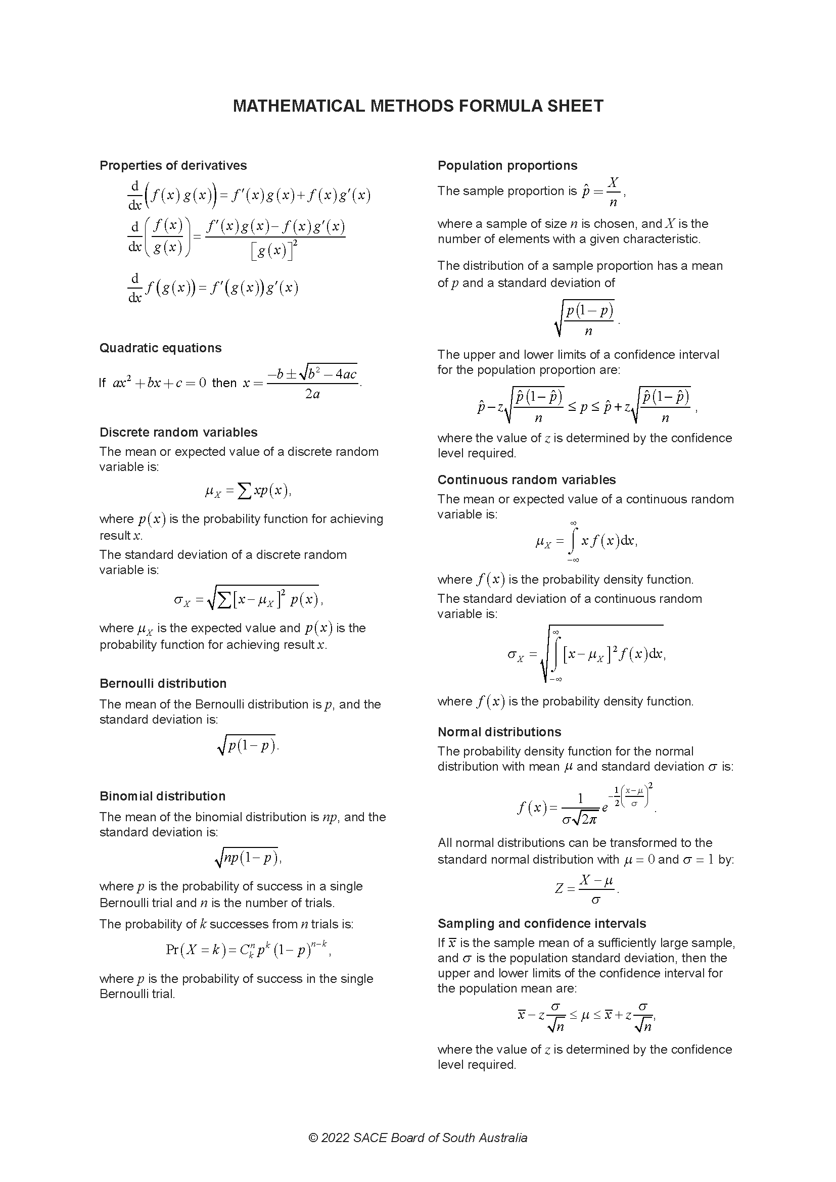
Let the random variable \(T\) represent the time, measured in minutes, for a randomly chosen customer to receive their order after placing it at a 24-hour fast-food restaurant. \(T\) can be modelled using the probability density function \[ f(t) = 0.3e^{-0.3t}, \text{ where } t \ge 0. \] A graph of \(y = f(t)\) is shown in Figure 1.
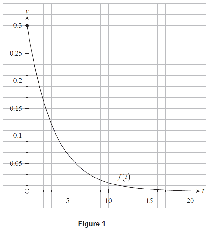
Figure 1
(a) (i) Calculate \(\int_2^5 f(t) \, dt\). (1 mark)
(ii) Interpret your answer to part (a)(i) in the context of receiving an order at the fast-food restaurant. (1 mark)
(b) (i) Determine the probability that a randomly chosen customer receives their order in less than 5 minutes, according to the model. (1 mark)
(ii) On Figure 1, represent the probability calculated in part (b)(i). (1 mark)
(c) Determine \(\int 0.3e^{-0.3t} \, dt\). (1 mark)
(d) The probability that a randomly chosen customer receives their order in less than \(r\) minutes is 0.8, according to the model. Using your answer to part (c), determine the exact value of \(r\). (3 marks)
Consider the function \(f(x) = kx^2 + 1\), where \(k\) is a non-zero constant.
(a) Using first principles, show that \(f'(x) = 2kx\). (3 marks)
Figure 2 shows the graph of \(y = f(x)\) for a certain value of \(k\). The tangent to the graph at \(x=2\) is also shown. This tangent has a \(y\)-intercept at \(A\).
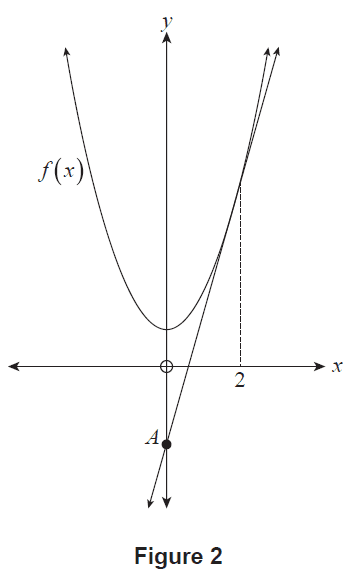
Figure 2
(b) Show that the tangent to the graph of \(y=f(x)\) at \(x=2\) has the equation \(y = 4kx - 4k + 1\). (3 marks)
(c) If the \(y\)-coordinate of \(A\) is \(-11\), determine the value of \(k\). (1 mark)
Astro Cats cards are a type of trading card. Among ordinary Astro Cats cards, gold cards can be found by chance. The probability that a single randomly selected card is a gold card is 0.035. The trading cards are sold in packs of 10 randomly selected cards.

(a) Assume that the number of gold cards found in packs of cards can be modelled using a binomial distribution.
(i) For one randomly selected pack of cards, calculate the:
(1) expected number of gold cards. (1 mark)
(2) probability of finding exactly one gold card. (1 mark)
(3) probability of finding more than two gold cards. (2 marks)
(ii) A collector states that in 12 randomly selected packs of cards there is a 100% chance of finding at least one gold card. Calculate the relevant probability to show that the collector's statement is incorrect. (1 mark)
Packs of Astro Cats trading cards may also contain platinum cards. These cards are rare, and the manufacturer does not publicly state how many are made. However, a website claims that the proportion of platinum cards produced is no more than 0.004.
(b) To assess the accuracy of the website's claim, a collector investigated their 1200 packs of 10 cards and found that these packs contained 51 platinum cards. The collector's 1200 packs of 10 cards can be considered a random sample for the purposes of this question.
(i) Show that the proportion of platinum cards in this sample is 0.00425. (1 mark)
(ii) Calculate a 90% confidence interval for the proportion of all cards that are platinum cards. (2 marks)
(iii) Hence, at the 90% confidence level, does the confidence interval that you calculated in part (b)(ii) support the website's claim? Justify your answer. (2 marks)
(a) Consider the function \(f(x) = \frac{2}{x-1} + 2x\), where \(x \ne 1\). A graph of \(y=f(x)\) is shown in Figure 3, with its two stationary points shown at \(A\) and \(B\).
Figure 3
(i) Show that \(f'(x) = \frac{2x^2 - 4x}{(x-1)^2}\). (3 marks)
(ii) Hence, use an algebraic approach to show that \(f(x)\) has exactly two stationary points, at \(x=0\) and \(x=2\). (2 marks)
(b) Consider the function \(g(x) = \frac{2}{x-m} + 2x\), where \(m\) is a constant and \(x \ne m\).
(i) Complete the following table for each given value of \(m\). (2 marks)
| \(m\) | Function | \(x\)-coordinates of the two stationary points of the function \(g(x)\) |
|---|---|---|
| 1 | \(g(x) = \frac{2}{x-1} + 2x\) | \(x=0, x=2\) |
| 2 | \(g(x) = \frac{2}{x-2} + 2x\) | |
| 3 | \(g(x) = \frac{2}{x-3} + 2x\) | |
| 4 | \(g(x) = \frac{2}{x-4} + 2x\) |
(ii) Make a conjecture about the \(x\)-coordinates of the two stationary points of the function \(g(x) = \frac{2}{x-m} + 2x\). (1 mark)
(iii) Prove or disprove your conjecture. (4 marks)
Consider the graph of the function \(y=f(x)\) shown in Figure 4 where \(f(x)\) is defined for all real values of \(x\). This function has exactly:
- two stationary points, located at \(B(b, f(b))\) and \(D(d, f(d))\)
- two inflection points, located at \(A(a, f(a))\) and \(C(c, f(c))\)
- two \(x\)-intercepts, located at \(B(b, f(b))\) and \(E(e, f(e))\).
As \(x\) increases for \(x > d\), the slope of \(f(x)\) approaches \(k\), where \(k < 0\). Additionally, \(f''(x)=0\) only at \(x=a\) and \(x=c\).
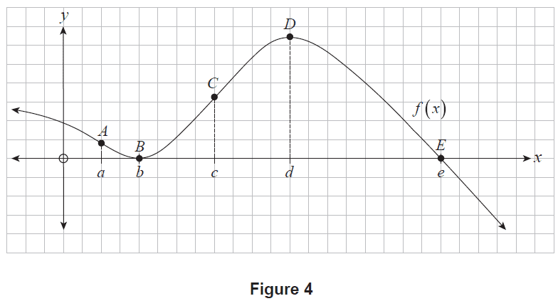
Figure 4
(a) Complete the sign diagram below for \(f'(x)\). (2 marks)
\(f'(x)\)
(b) (i) Which one statement is true? Tick the appropriate box to indicate your answer. (1 mark)
\(f'(0) < f'(a)\)
\(f'(0) = f'(a)\)
\(f'(0) > f'(a)\)
(ii) Which one statement is true? Tick the appropriate box to indicate your answer. (1 mark)
\(f(d) < 0\) and \(f''(d) < 0\)
\(f(d) < 0\) and \(f''(d) > 0\)
\(f(d) > 0\) and \(f''(d) < 0\)
\(f(d) > 0\) and \(f''(d) > 0\)
(c) State the interval(s) of \(x\) for which \(f''(x) \ge 0\). (1 mark)
(d) On Figure 5, sketch a possible graph of \(y=f'(x)\). Note that \(k\) has been added to the \(y\)-axis. (3 marks)
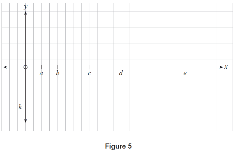
Figure 5
The daily milk production of a randomly chosen milking cow varies, and can be modelled by a normal distribution with a mean of \(\mu = 21.9\) litres and a standard deviation of \(\sigma = 3.26\) litres.

(a) (i) Determine the probability that the daily milk production of a randomly selected cow is less than 23 litres. (1 mark)
(ii) Given that 15% of randomly selected cows have a daily milk production of \(c\) litres or more, determine the value of \(c\). (1 mark)
(b) Let the random variable \(S_n\) represent the total daily milk production of a random sample of \(n\) cows. Explain why it is appropriate to model \(S_n\) using a normal distribution. (1 mark)
Recall that the daily milk production of a randomly chosen milking cow can be modelled by a normal distribution with a mean of \(\mu=21.9\) litres and a standard deviation of \(\sigma=3.26\) litres.
(c) Let the random variable \(S_{90}\) represent the total daily milk production of a random sample of 90 cows.
(i) Show that the mean of \(S_{90}\) is \(\mu_{S_{90}} = 1971\) litres and standard deviation of \(S_{90}\) is \(\sigma_{S_{90}} = 30.93\) litres (correct to four significant figures). (2 marks)
(ii) Determine the probability that the total daily milk production of a random sample of 90 cows is:
(1) between 1900 litres and 1950 litres. (1 mark)
(2) more than 2000 litres. (1 mark)
A farmer owns 90 cows, which can be considered a random sample for the purposes of this question. The farmer aims to increase their cows' total mean daily milk production by adopting a new feeding plan for the cows. The farmer randomly selects 20 cows for the new feeding plan. In this random sample of 20 cows, the mean daily milk production after some time on the new feeding plan is 23.5 litres per cow.
(d) Calculate a 95% confidence interval for the mean daily milk production per cow on the new feeding plan. Assume that the standard deviation is still \(\sigma = 3.26\) litres. (2 marks)
(e) Does the confidence interval calculated in part (d) suggest with 95% confidence that the new feeding plan has increased the mean daily milk production per cow? Justify your answer. (2 marks)
(f) The farmer would like the 90 cows' mean total daily milk production to be more than 2000 litres.
(i) Determine the mean daily milk production per cow if 90 cows had a total daily milk production of 2000 litres. (1 mark)
(ii) Hence or otherwise, does the confidence interval calculated in part (d) suggest with 95% confidence that the new feeding plan will result in the 90 cows' mean total daily milk production being more than 2000 litres? Justify your answer. (2 marks)
A self-balancing robot uses a device called a PID controller to stop itself from falling over after being placed on its wheels and released. Let \(L(t)\) represent the angle of lean of the robot, at \(t\) seconds after release, where \(L(t)\) is measured in radians. Side-on diagrams of this robot in Figure 6 show various angles of lean, where:
- negative values of \(L(t)\) mean the robot has an angle of lean to the left
- \(L(t) = 0\) means the robot is vertical
- positive values of \(L(t)\) mean the robot has an angle of lean to the right.
This image cannot be reproduced here for copyright reasons.
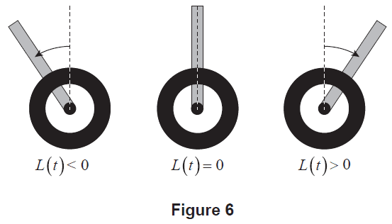
Figure 6
The PID controller's settings can be adjusted to change how long it takes the robot to reach an approximately stable vertical position after initially being placed on its wheels and released. Engineers conducted an experiment using different settings on the PID controller, starting with Setting A.
(a) Using Setting A, the robot was initially placed on its wheels and released. The resulting angle of lean was recorded for 6 seconds. Using this setting, the angle of lean of the robot, \(L(t)\), at \(t\) seconds after release, can be modelled by the function \[ L(t) = 0.75e^{-0.75t} \cos(4t), \text{ where } 0 \le t \le 6. \] A graph of \(y=L(t)\) for Setting A is shown in Figure 7.
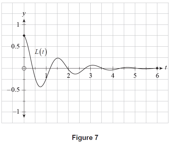
Figure 7
(i) State the initial angle of lean of the robot, according to the model. (1 mark)
(ii) Determine the value of \(L'(1.3)\). (1 mark)
(iii) Interpret your answer to part (a)(ii) in the context of the problem, stating the appropriate units. (2 marks)
(iv) Calculate how long after being released the robot is leaning to the left with its maximum angle, according to the model. (1 mark)
(b) The engineers were not satisfied with how long the robot took to reach an approximately stable vertical state using Setting A. To improve results, the experiment was repeated using Setting B and the same initial angle of lean. Using Setting B, the angle of lean of the robot, \(L(t)\), at \(t\) seconds after release, can now be modelled by the new function \[ L(t) = 0.75e^{-t} \cos t, \text{ where } 0 \le t \le 6. \] A graph of \(y=L(t)\) for Setting B is shown in Figure 8.
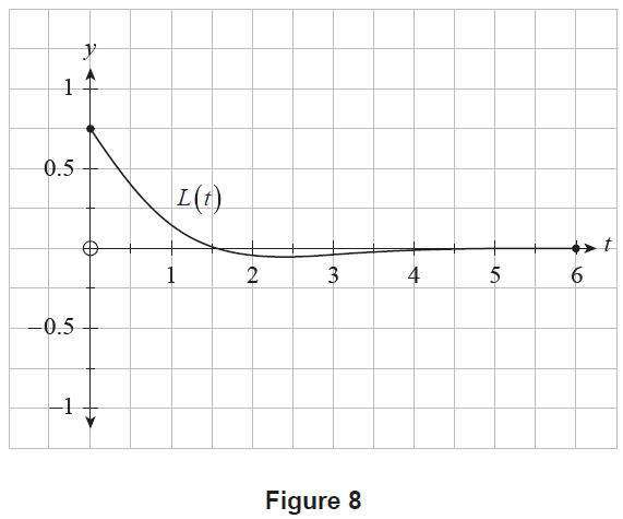
Figure 8
(i) Determine \(L'(t)\) for Setting B. (2 marks)
(ii) Hence, for Setting B, use an algebraic approach to determine the exact values of \(t\) such that \(L'(t)=0\), during the first 6 seconds after release. (3 marks)
Consider a discrete random variable, \(X\), which has the probability mass function \[ \Pr(X=x) = \frac{e^{-2}2^x}{x!} \] where \(x\) is a non-negative integer, and \(x! = x \times (x-1) \times (x-2) \times \dots \times 3 \times 2 \times 1\) with \(0!=1\).
(a) Based on the information provided, complete the table below by calculating the missing probabilities. State your answers correct to four decimal places. (2 marks)
| \(\Pr(X=0)\) | \(\Pr(X=1)\) | \(\Pr(X=2)\) | \(\Pr(X=3)\) | \(\Pr(X=4)\) | \(\Pr(X=5)\) | \(\Pr(X \ge 6)\) |
| 0.2707 | 0.2707 | 0.1804 | 0.0902 | 0.0166 |
A moment-generating function can be used to find key properties of a distribution without using the probability mass function directly. For the probability mass function given above, the moment-generating function is \[ M(t) = e^{2e^t-2}. \]
(b) The mean, \(\mu\), of the probability mass function given above can be found using the formula \[ \mu = M'(0). \] Show that \(\mu=2\). (2 marks)
(c) (i) Show that \(M''(t) = 2e^{2e^t-2}(2e^{2t}+e^t)\). (2 marks)
(ii) The standard deviation, \(\sigma\), of the probability mass function given above can be found using the formula \[ \sigma = \sqrt{M''(0) - \mu^2}. \] Show that \(\sigma = \sqrt{2}\). (2 marks)
(d) Hence, determine the probability that \(X\) is within one standard deviation of the mean. (2 marks)
Consider the function \(f(x) = \ln(2(x+1)^2)\) for \(x > -1\). The graph of \(y=f(x)\) is shown in Figure 9.
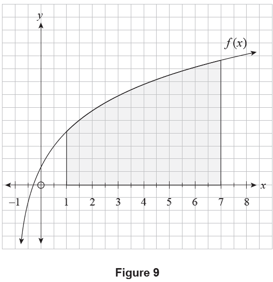
Figure 9
Let \(A\) be the area bounded by the graph of \(y=f(x)\), the \(x\)-axis, and the vertical lines at \(x=1\) and \(x=7\). In Figure 9, \(A\) is represented by the shaded region.
(a) Let \(U_3\) represent an upper estimate of \(A\) using the areas of three rectangles of equal width.
(i) On Figure 9, draw three rectangles that can be used to calculate \(U_3\). (1 mark)
(ii) Hence, calculate the value of \(U_3\). (2 marks)
(iii) Write an integral expression for the exact value of \(A\). (1 mark)
(b) Consider the function \(y=x\ln x\), where \(x > 0\).
(i) Find \(\frac{dy}{dx}\). (1 mark)
(ii) Using your result from part (b)(i), show that \[ \int \ln(2x^2) \, dx = x(\ln(2x^2) - 2) + c, \] where \(c\) is a real constant and \(x > 0\). (4 marks)
Consider the functions \(f(x) = \ln(2(x+1)^2)\) for \(x > -1\) and \(g(x) = \ln(2x^2)\) for \(x>0\). The graphs of \(y=f(x)\) and \(y=g(x)\) are shown in Figure 10.
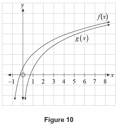
Figure 10
(c) Describe the relationship between the graphs of \(y=f(x)\) and \(y=g(x)\). (1 mark)
(d) The exact value of \(A\) (i.e. the area bounded by the graph of \(y=f(x)\), the \(x\)-axis, and the vertical lines at \(x=1\) and \(x=7\)) can be calculated using a definite integral. Use part (b)(ii) and your answer to part (c) to determine the exact value of \(A\). Express your answer in the form \(p \ln 2 + q\), where \(p\) and \(q\) are integers. (4 marks)
end of booklet
SACE is a registered trademark of the South Australian Certificate of Education. The SACE does not endorse or make any warranties regarding this study resource. Past SACE exams and related content can be accessed directly at www.sace.sa.edu.au.