2024 SACE Stage 2 Maths Methods Exam Paper

Question 1 (9 marks) [2024 Question 1]

Let \(X\) be a normally distributed random variable with a mean of \(\mu = 54\) and a standard deviation of \(\sigma = 6\).

(a) Determine

(i) \(\Pr(50 \le X \le 52)\). (1 mark)

(ii) \(\Pr(X \ge 58)\). (1 mark)

(b) Given that \(\Pr(X \ge k) = 0.10\), determine the value of \(k\). (1 mark)

Figure 1 shows the graph of the probability density function for the random variable \(X\). The dashes on the \(x\)-axis show increments of one standard deviation.

(c) On Figure 1, write a number in each box to provide a scale for the \(x\)-axis. (2 marks)

(d) Let \(\bar{X}_4\) be the random variable representing the sample mean of 4 independent observations of \(X\).

(i) State the mean and standard deviation of \(\bar{X}_4\). (2 marks)

(ii) On Figure 1 above, sketch the probability density function for the random variable \(\bar{X}_4\). (2 marks)

Question 2 (9 marks) [2024 Question 2]

Car A and Car B are toy cars powered by compressed carbon dioxide. After they are released from a starting point, the cars travel only forwards in a straight line, and are observed for exactly 2 seconds.

Car A's velocity \(t\) seconds after it is released, \(v_A(t)\), can be modelled using the function \[ v_A(t) = 3e^{1.5t} - 3 \] where \(v_A(t)\) is measured in metres per second and \(t\) is measured in seconds for \(0 \le t \le 2\).

(a) Determine Car A's velocity 1 second after it is released. (1 mark)

(b) Let \(s_A(t)\) be a function that models the displacement of Car A from the starting point \(t\) seconds after it is released.

(i) Show that \(s_A(t) = 2e^{1.5t} - 3t - 2\). Assume that \(s_A(0) = 0\). (2 marks)

(ii) Hence or otherwise, determine the displacement of Car A from the starting point 2 seconds after it is released. (1 mark)

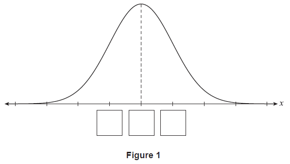
The graph of \(y = v_A(t)\) is shown in Figure 2.

Car B's velocity \(t\) seconds after it is released, \(v_B(t)\), can be modelled using the function \[ v_B(t) = 6.6t^2 + 8t \] where \(v_B(t)\) is measured in metres per second and \(t\) is measured in seconds for \(0 \le t \le 2\).

(c) On Figure 2 above, sketch the graph of \(y = v_B(t)\). (2 marks)

(d) For what values of \(t\) was the velocity of Car A greater than the velocity of Car B? (1 mark)

(e) Which car, Car A or Car B, do the models suggest has travelled the furthest during the 2 seconds that they are observed? Justify your answer. (2 marks)

Question 3 (6 marks) [2024 Question 3]

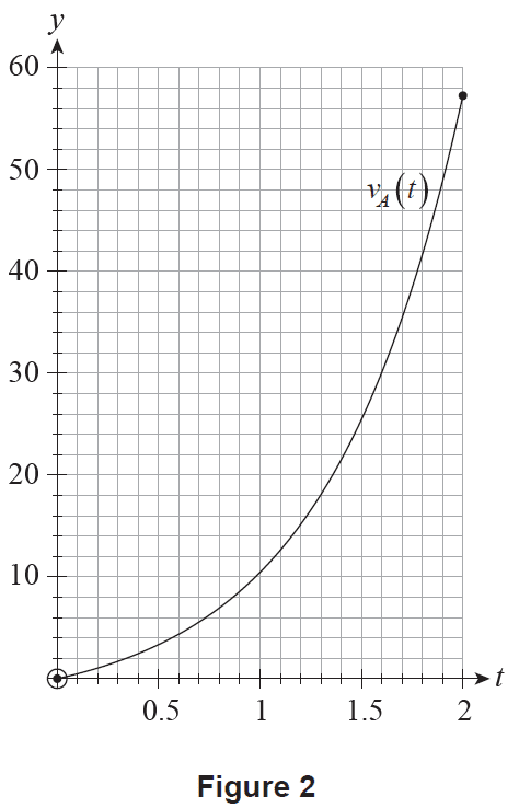
Consider the function \(f(x) = \ln(x+3)\) where \(x > -3\). A graph of \(y = f(x)\) is shown in Figure 3.

(a) Determine \(f'(x)\). (1 mark)

(b) Calculate \(f'(0)\). (1 mark)

Let \(g(x) = b\ln(x+3)\), where \(x > -3\) and \(b\) is a positive constant.
Figure 4 shows the graph of \(y=f'(x)\) and \(y=g'(x)\). The \(y\)-intercepts of each graph are labelled \(A\) and \(B\) respectively.

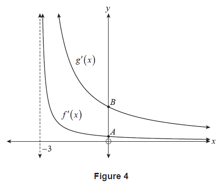
(c) The vertical distance between points \(A\) and \(B\) is 2 units. Determine the value of \(b\). (3 marks)

(d) Hence or otherwise, state the transformation applied to \(f(x)\) to obtain \(g(x)\). (1 mark)

Question 4 (12 marks) [2024 Question 4]

(a) Consider a scenario where a random sample size of 100 is taken and 23 successes are observed.

(i) Fill in the boxes below to form a 95% confidence interval for the population proportion of successes, \(p\).

  \(\le p \le\)   (1 mark)

(ii) Does the confidence interval calculated in part (a)(i) contradict the statement that \(p = 0.35\) with 95% confidence? Tick the appropriate box to indicate your answer. (1 mark)

Yes No

(iii) Justify your answer to part (a)(ii). (1 mark)

(b) A mathematician is demonstrating that not all calculated confidence intervals will contain the population proportion being investigated.

The mathematician uses a population that is known to have a population proportion of 0.35. They take 50 independent, randomly generated samples of size 100 and calculate 50 independent 95% confidence intervals.

Figure 5 shows these confidence intervals as vertical lines, where the vertical position of the endpoints of each line represents the limits of each confidence interval. Each confidence interval has been assigned a label from 1 to 50.

The population proportion of 0.35 is represented as a horizontal dashed line.

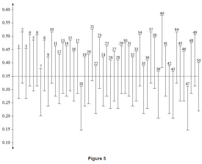
(i) Identify the assigned labels of the three confidence intervals that do not contain the population proportion. (1 mark)

(ii) Identify the assigned label(s) of the confidence interval(s) that could be used to support a claim that the population proportion is greater than 0.35. (1 mark)

When a 95% confidence interval for a population proportion is to be calculated using a random sample of sufficient size, there is a probability of 0.05 that the confidence interval will not contain the population proportion.

(c) Let \(X\) be the number of 95% confidence intervals that will not contain the population proportion out of 100 independent 95% confidence intervals to be calculated.

(i) Assuming that \(X\) can be modelled using a binomial distribution, fill in the boxes below to show the value of the parameters of \(X\). (2 marks)

\(X \sim B(\)   ,   \( ) \)

(ii) If 100 new, independent 95% confidence intervals are to be calculated, determine the probability of observing:

(1) exactly five 95% confidence intervals that will not contain the population proportion. (1 mark)

(2) at least one 95% confidence interval that will not contain the population proportion. (1 mark)

(d) Determine the minimum number of independent 95% confidence intervals that would need to be calculated to have a greater than 0.5 probability of having at least one 95% confidence interval that will not contain the population proportion. (3 marks)

Question 5 (5 marks) [2024 Question 5]

Consider the function \(f(x) = \frac{x}{x-2}\), where \(x \ne 2\).

(a) Use first principles to find \(f'(x)\). (4 marks)

(b) Hence or otherwise, state the slope of the tangent to \(f(x)\) when \(x=6\). (1 mark)

Question 6 (12 marks) [2024 Question 6]

(a) Use an algebraic approach to show that \(k = \frac{1}{\ln 1.1}\). (3 marks)

(b) (i) Calculate \(\int_{400}^{410} \frac{1}{(\ln 1.1)x} \,dx\). (1 mark)

(ii) Interpret your answer to part (b)(i) in the context of the problem. (1 mark)

(c) Show that the mean of \(X\) is \(\mu_X = \frac{40}{\ln 1.1}\) grams. (3 marks)

(d) The company alters the stopping mechanism in order to reduce the amount of excess sand in the bags.

After the stopping mechanism has been altered, they take a random sample of 25 bags of sand and find that the mean net weight of the sand in these bags is 417 grams. Assume that the standard deviation is \(\sigma_X = 11.5\) grams and the sample size is large enough for the central limit theorem to apply.

(i) Calculate the 99% confidence interval for the mean net weight of the sand in the bags after the stopping mechanism was altered. (2 marks)

(ii) The company claims that after the stopping mechanism was altered, the mean net weight of the sand in the bags has reduced. Does the confidence interval calculated in part (d)(i) support this claim with 99% confidence? Justify your answer. (2 marks)

Question 7 (10 marks) [2024 Question 7]

Consider the function \(f(x) = \frac{1}{x^2}\).

(a) Use an algebraic approach to determine the equation of the tangent to \(f(x)\) at \(x=1\). (3 marks)

(b) Determine the \(x\)-intercept of this tangent. (1 mark)

Consider the function \(g(x) = \frac{1}{x^2+k}\), where \(k\) is a non-negative constant. The \(x\)-intercept of the tangent to \(g(x)\) at \(x=1\) is shown in Table 1 for various values of \(k\).

Table 1

\(k\)	1	2	3	4
\(g(x)\)	\(\frac{1}{x^2+1}\)	\(\frac{1}{x^2+2}\)	\(\frac{1}{x^2+3}\)	\(\frac{1}{x^2+4}\)
\(x\)-intercept of the tangent to \(g(x)\) at \(x=1\)	\((2,0)\)	\(\left(\frac{5}{2}, 0\right)\)	\((3,0)\)	\(\left(\frac{7}{2}, 0\right)\)

(c) Make a conjecture about the \(x\)-intercept of the tangent to \(g(x) = \frac{1}{x^2+k}\) at \(x=1\). (1 mark)

(d) Prove or disprove the conjecture that you made in part (c). (5 marks)

Question 8 (12 marks) [2024 Question 8]

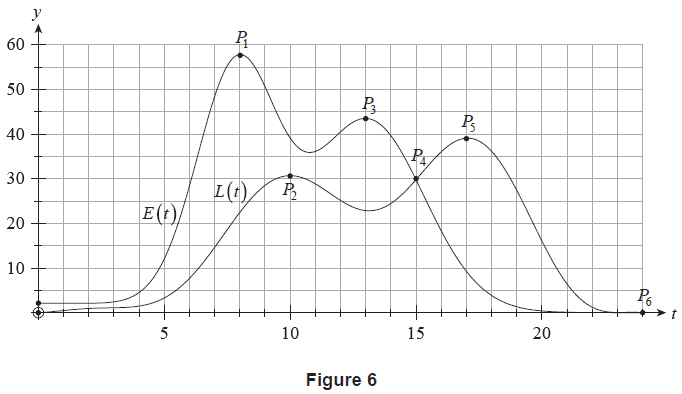
The \(t\)-coordinates of the labelled points and the values of various integral expressions are shown in Table 2. Assume that \(P_1\), \(P_2\), \(P_3\), and \(P_5\) are stationary points.

Table 2

Point \(P_i\)	\(P_1\)	\(P_2\)	\(P_3\)	\(P_4\)	\(P_5\)	\(P_6\)
\(t_i\), the \(t\)-coordinate of \(P_i\)	8	10	13	15	17	24
\(\int_{0}^{t_i} E(t)dt\)	130	230	347	429	462	471
\(\int_{0}^{t_i} L(t)dt\)	40	96	177	227	298	406

(a) (i) It is known that \(E'(9) = 50.6\). State the meaning of this result in the context of the problem. (2 marks)

(ii) Use the information given on page 4 to determine:

(1) how many hours after midnight vehicles were leaving Park-o-Rama at the maximum rate. (1 mark)

(2) how many vehicles entered Park-o-Rama during the 24-hour period. (1 mark)

(3) how many vehicles left Park-o-Rama during the final 7 hours of the day. (1 mark)

(iii) The maximum number of vehicles in Park-o-Rama was 202. How many hours after midnight did this occur? (1 mark)

(b) Recently, more people have started driving electric vehicles (EVs).

In 2024, one study found that:

• • non-EVs have an average weight of 2.25 tonnes
• • EVs are 36% heavier than non-EVs
• • 7% of vehicles are EVs.

(i) Use the information given above to complete Table 3. (2 marks)

Table 3

	Non-EVs	EVs
Weight (tonnes)	2.25
Proportion of vehicle type		0.07

Let \(X\) represent the weight in tonnes of a randomly selected vehicle in 2024.

(ii) Use the information in Table 3 to show that \(X\) has a mean of \(\mu_X = 2.31\) tonnes (correct to three significant figures). (1 mark)

The engineers working for Park-o-Rama are studying the day considered on page 4. They would be concerned if the total weight of vehicles in Park-o-Rama exceeds 475 tonnes with a probability greater than 0.005 at any point during the day.

(iii) Determine whether the engineers would be concerned. Assume that your chosen sample size is large enough for the central limit theorem to apply, the vehicles in Park-o-Rama constitute a random sample of vehicles, and that the weights of the vehicles, \(X\), have \(\mu_X = 2.31\) and \(\sigma_X = 0.207\) tonnes. (3 marks)

Question 9 (12 marks) [2024 Question 9]

(a) Consider the functions \(f(x) = e^x - 4e^{2x}\) and \(g(x) = e^{3x} - 4e^{2x}\). Figure 7 shows the graph of \(y=f(x)\) and Figure 8 shows the graph of \(y=g(x)\) with the stationary point of each function labelled as \(P\) and \(Q\) respectively.

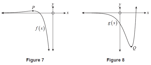
Complete Table 4 below by finding the \(y\)-coordinates of \(P\) and \(Q\). (2 marks)

Table 4

Point	\(y\)-coordinate
\(P\)
\(Q\)

(b) Consider the function \(y = e^{ax} - 4e^{2x}\) where \(a\) is a positive constant such that \(a \ne 2\).

(i) Show that the \(x\)-coordinate of the only stationary point of \(y = e^{ax} - 4e^{2x}\) is \(x = \frac{1}{a-2}\ln\left(\frac{8}{a}\right)\). (4 marks)

(ii) (1) Show that the \(y\)-coordinate of the stationary point of \(y = e^{ax} - 4e^{2x}\) is \(y = 4\left(\frac{8}{a}\right)^{\frac{2}{a-2}}\left(\frac{2-a}{a}\right)\). (4 marks)

(2) Determine the values of \(a\) for which the \(y\)-coordinate of the stationary point of the function \(y = e^{ax} - 4e^{2x}\) is positive. Justify your answer. (2 marks)

Question 10 (13 marks) [2024 Question 10]

Consider the function \(f(x) = e^{-\cos x}\) for \(0 \le x \le 2\pi\) with derivative \(f'(x) = e^{-\cos x}\sin x\). Figure 9 shows the graph of \(y=f(x)\) and \(y=f'(x)\). The two functions touch at \(P\).

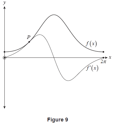
(a) Use an algebraic approach to determine the exact \(x\)-coordinate of \(P\). (3 marks)

Recall that \(f(x) = e^{-\cos x}\) for \(0 \le x \le 2\pi\) with derivative \(f'(x) = e^{-\cos x}\sin x\).

(b) (i) Show that \(f''(x) = e^{-\cos x}(-\cos^2 x + \cos x + 1)\).
Note that \(\cos^2 x + \sin^2 x = 1\). (2 marks)

(ii) Hence, use an algebraic approach to determine the values of \(x\) such that \(f''(x) = f(x)\). (3 marks)

Figure 10 shows the graph of \(y=f'(x)\) and \(y=f''(x)\), which intersect when \(x=k\) and at one other point. The two distinct regions enclosed between the two functions from \(x=k\) to \(x=2\pi\) are denoted as \(A\) and \(B\), as shown in Figure 10. The areas of these regions are measured in units squared.

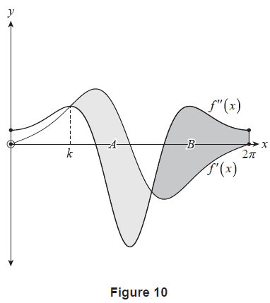
(c) Use part (a) and part (b)(ii) to explain why \(k = \frac{\pi}{2}\). (1 mark)

(d) Use an algebraic approach to determine the exact difference in area between region \(A\) and region \(B\). (4 marks)